Remember Magic Avatars in the Lensa app that were all the rage a few months ago? The custom AI generated avatars from just a few photos of your face were a huge hit!
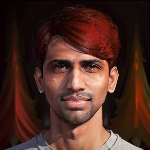
 Reference portrait image of me
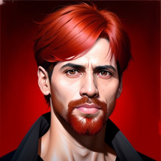
![]() One of my Lensa “Magic Avatars”
One of my Lensa “Magic Avatars”
The technology behind this product is the open source Stable Diffusion image generation model. You can run this model on your own computer, on a cloud GPU instance, or even a free colab notebook — to generate your own avatars. In this post I’ll walk you through the process of doing exactly that!
Before diving in, it would help to review the AI Primer: Image Models 101 post if you are new to the world of image models in general. I also wrote a quick guide on getting Stable Diffusion set up on your computer — I’ll assume you’ve already done that.
What is fine-tuning?
I previously argued that one of the main advantages Stable Diffusion has over a proprietary model like Midjourney is the ability to customize it. While Midjourney produces stunning imagery with very little effort, it is going to have a difficult time producing photos of your likeness or in a niche style. This is getting better with their image-to-image features, but for any work requiring a high degree of flexibility and control, it is hard to beat Stable Diffusion’s capabilities.
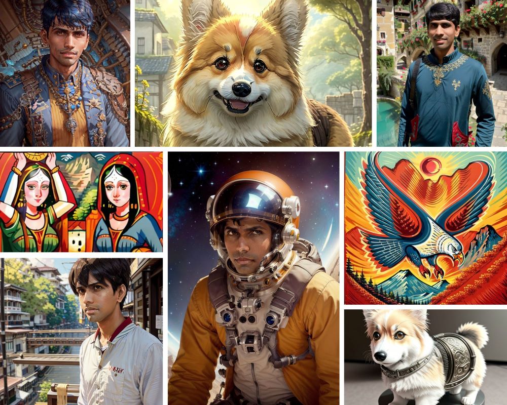 Examples of AI-generated images with Stable Diffusion, after fine-tuning
This level of customization is unlocked by the concept of fine-tuning. At a high level, fine-tuning is the process of taking a large pre-trained model and training it on your own data to achieve a specific result. This process is becoming increasingly popular in the ML community as the pre-trained models get larger and much more capable. It provides the last mile tuning you need to get dramatically improved performance on your specific problem — with much less effort than it would take to build a whole new model from scratch.
Fine-tuning has been successfully applied in many realms such as ChatGPT and Alpaca for text. In the image generation space, it is typically used to teach models to generate images featuring custom characters, objects, or specific styles — especially those that the large pre-trained model has not encountered before.
Types of fine-tuning
The classic way to fine-tune image models is conceptually simple: provide a large dataset of labeled image and caption pairs; then re-run training using the existing model weights as a prior. This process is very similar to how the pre-trained model learned concepts in the first place. Lambda Labs wrote very good article on how they produced the “text-to-pokemon” model by doing this.
This type of fine-tuning, while substantially cheaper and easier to do than building a new model from scratch, still requires a lot of data (on the order of hundreds of images) and GPU compute time. Since then, there have been many innovative techniques published by researchers on how to make this process even more effective and efficient. I’ll briefly touch on the three most popular ones:
Textual inversion
This paper from researchers at Tel Aviv University and NVIDIA proposed a way to learn a new concept from as little as 3-5 example images, and notably does not require changing the base pre-trained model in any way. I won’t go into the details of how this works here, but paperspace has a good tutorial on this process, and there is a page maintained in the Automatic1111 UI Wiki on how to use and train using textual inversion.
The ultimate output of this process is a very small “embeddings” file that is typically less than 100 kilobytes. This embedding can be used in tandem with the base model to generate the learned concepts in new ways.
Dreambooth
This paper from researchers at Google also only requires 3-5 example images and is able to learn a new character or style. However, Dreambooth does this by directly modifying the pre-trained models and updates the weights. This is a more powerful technique, but the output of the process is a whole new model that is roughly the same size as the pre-trained one. For Stable Diffusion 1.5 that means your newly produced model will be around 4.5 gigabytes!
There is evidence to suggest that commercial products like Lensa’s Magic Avatars uses this technique with great results. Replicate has a good blog post on how to train a model using Dreambooth, and their service makes it easy to make one if you don’t have access to a powerful GPU.
LoRA
This type of fine-tuning is based on the paper “Low-Rank Adaptation of Large Language Models” — which as the name suggests — was originally a technique used to fine-tune large language models like GPT-3.
While the general technique predates both Textual Inversion and Dreambooth, its application to diffusion models for image generation is very new, kicked off by early this year by cloneofsimo. This method produces an output that is between 50 and 200 megabytes in size, and does not require modifying the pre-trained model.
Pros & Cons
Let’s summarize these three techniques.
| Type | # of Examples | Output Size | Notes |
|---|---|---|---|
| Textual Inversion | 3-5 minimum, ideally 20-30 | < 100 KB embeddings file | OK quality, works better for remixing of existing concepts in the base model. You can combine multiple embeddings at runtime to generate multiple concepts, a single embedding usually represents a single concept or style. |
| Dreambooth | 3-5 minimum, ideally 20-30 | ~4.5 GB full model | Great quality, works well for both characters and styles. Since it produces a new full model, you have to train multiple characters in a single training. Mixing styles can be tricky to accomplish. |
| LoRA | 20-50 for characters, 50-200 for styles | ~50-200 MB tensor files | Good quality, somewhere between Textual Inversion and Embeddings. You can apply multiple LoRAs at runtime (just like embeddings) and are very flexible to mix and match. |
Note: I won’t discuss another technique called “hypernetworks” here (this is NOT the same as the technique popularized by this 2016 paper), primarily because vetted knowledge of how to make one optimally is hard to come by.
In this tutorial, I will focus on the LoRA fine-tuning technique. In my own experimentation, I’ve found it gave me results that were higher quality than textual inversion, but with an output not as heavyweight as Dreambooth. This let me build a number of characters and styles fairly quickly.
Basics of a LoRA setup
Training a LoRA model itself takes only around 10 minutes, but expect the whole process including setting up and preparing training data to take around 2 hours.
There are two main options you have for LoRA training. The original implementation by cloneofsimo seems to have worked well for many, however, I had two issues with it:
- The default parameters did not work well with my own training data.
- The output of this implementation is not compatible with the Automatic1111 UI (that I recommended in my post on Installing Stable Diffusion). If you do want to try out this original implementation, replicate once again has an easy step-by-step tutorial on how to do it.
I opted for kohya’s implementation because it produces outputs compatible with the Automatic1111 UI and offers additional options for adjusting the fine-tuning process. I ran this locally on my (brand new!) RTX 4090, but the process can be run on a machine with as little as 6 GB of VRAM. This guide is focused on fine-tuning locally with an NVIDIA card. If you don’t have one, you can use Google Colab to train your models, which has a generous free tier - this notebook uses much of the same techniques I’ll talk about here.
There is very handy UI wrapper on top of kohya’s training scripts called kohya_ss that we will be using. It makes it easier to manage various configurations and has some nice utilities like auto-captioning that will come in handy.
We’ll use pyenv again to manage our Python environment. Let’s make a new one for the kohya_ss GUI, as the requirements here differ slightly from the ones needed for the Automatic1111 UI.
$ pyenv install 3.10.10
$ git clone [email protected]:bmaltais/kohya_ss.git
$ cd kohya_ss
$ pyenv local 3.10.10
Now, let’s install the requirements for the GUI and training scripts. Execute in this specific order, so you have the most optimized version of pytorch (you basically want the one with CUDA 11.8 support):
$ pip install -r requirements.txt
$ pip install torch torchvision --extra-index-url https://download.pytorch.org/whl/cu118
$ pip install -U xformers
Finally, let’s configure accelerate. The defaults work just fine, the only setting that I changed was to use bf16 for mixed precision. All Ampere architecture cards (RTX 3000 or higher) support this format, which results in speedier training runs. Use fp16 if you care about backward compatibility, e.g. you want to run inference on your fine-tuned model on cards that don’t support bf16.
$ accelerate config

In which compute environment are you running?
This machine

Which type of machine are you using?
No distributed training

Do you want to run your training on CPU only (even if a GPU is available)? [yes/NO]:
NO

Do you wish to optimize your script with torch dynamo?[yes/NO]:
NO

Do you want to use DeepSpeed? [yes/NO]:
NO

What GPU(s) (by id) should be used for training on this machine as a comma-seperated list? [all]:
all

Do you wish to use FP16 or BF16 (mixed precision)?
bf16
Let’s test that everything worked by starting the GUI:
# From the kohya_ss directory
$ python kohya_gui.py
Load CSS...
Running on local URL:  http://127.0.0.1:7860

To create a public link, set `share=True` in `launch()`.
Open up the printed URL in your browser. If that worked, we are ready to begin the process of fine-tuning. I’ll walk you through what I did to train a LoRA for my own face.
Training data preparation
Machine learning makes the age-old computer science concept of “Garbage in, garbage out” painfully obvious. Expect to spend a good chunk of time preparing your training data, this is time well-invested towards ensuring a good quality output! I can imagine this workflow getting more and more automated over time, but for now, we’ll have to do it manually.
Image selection
My first stop was Google Photos, where I grabbed the 50 most recent images that included my face. A few guidelines to keep in mind:
- Focus on high resolution, high quality images. If a photo is blurry or low resolution, err on the side of not including it in the training set.
- You need to be able to crop the photo such that you are the only face in the photo after doing the cropping.
- A good variety of close-up photos and some full-body shots are ideal. Avoid photos where you are really far away, there’s not much for the model to learn from these.
- Try to shoot for variety in terms of lighting, poses, backgrounds, and facial expressions. The greater the diversity, the more flexible your model will be.
Applying these guidelines, I got a set of 25 usable images. I then proceeded to crop them — the default Windows Photos tool worked great, birme is another useful online tool. Don’t worry about cropping to a specific size or aspect ratio, just crop so your face and/or body are the predominant entity in the image with some background detail but ideally no other people. Make sure all your cropped images are in a single directory and have unique names (excluding the file extension).
Captioning
The next step in the process is to caption each image. In my experiments, there was a marked difference in quality when training with captions compared to without, so I highly recommend doing this.
Fortunately, as I described in my image models primer post, you can use automated techniques to generate image descriptions, which can significantly reduce your workload! One of the reasons we are using the kohya_ss GUI instead of the original training scripts directly is for the captioning feature, so let’s fire that up.
Open up the printed URL in your browser, head over to the Utilities tab and BLIP Captioning. Use the following settings:
- Image folder to caption: should point to the directory containing the cropped images from the previous step.
- Caption file extension: the convention is to have a
.txtfile next to each image file containing the description for it. - Prefix to add to BLIP caption: it helps to prefix each description with
photo of <token>,— so the model learns to associate the token with your likeness. - Increase “Number of beams” to 10, and set “Min length” to 25, so you get captions with at-least two sentences.
The page should look something like this:
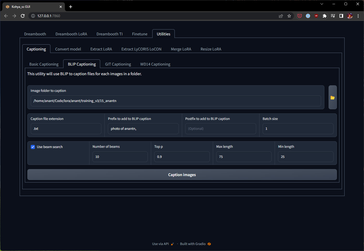
Click “Caption images” and let it run! Shouldn’t take more than a few minutes, you can review the progress on the command line where you launched kohya_gui.py.
Once the process is complete, open up the folder of training images where you should now see a .txt file with the same filename as each image. I would do a quick once over to make sure the captions are sensible, feel free to make edits and save them back to the same text file. Here are some general guidelines for good captions:
- Your goal is to associate your likeness with the token you chose. Characteristics that are the same in every photo (in my case, “black hair” and “brown skin”) should not be in the caption.
- Explicitly caption things that are different in each photo, e.g. “wearing sunglasses” or “wearing a white shirt”.
- Describe the type of photo, e.g. “close up” or “full body”.
- If the photo contains other elements such as a background, describe them as well, e.g. “in a kitchen” or “in a park”.
- If the photo was taken in the iPhone portrait mode, call it out, and include tags like “blurry background”.
Remember, the more accurate and descriptive your captions are, the easier it will be for the model to be flexible in image generation (e.g., swapping out black hair for purple hair).
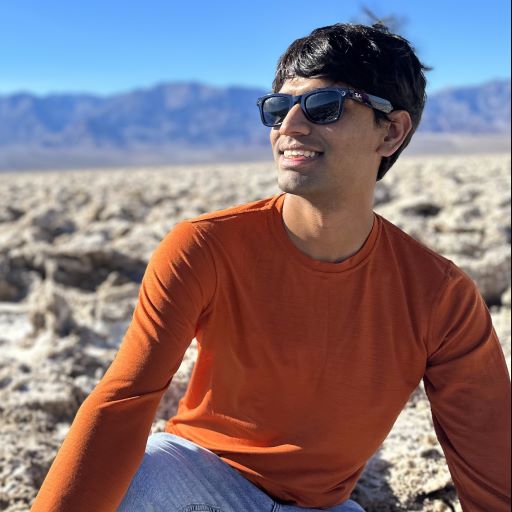 Example auto-generated caption: “photo of anantn, a man in an orange shirt and sunglasses sitting on a rock in the middle of the desert”
Hyperparameter selection
I spent a lot of time playing with the knobs you have at your disposal when fine-tuning. I’ll discuss the relevant hyperparameters in a more detail below, but if you’re just interested in the optimal configuration I found, jump ahead to the training section. In fact, I’d recommend you do that first, and then come back here to read about the hyperparameters to further refine your LoRA.
Training steps
The total number of training steps your fine-tuning run will take is dependent on 4 variables:
total_steps = (num_images * repeats * max_train_epochs) / train_batch_size
Your goal is to end up with a step count between 1500 and 2000 for character training. The number you can pick for train_batch_size is dependent on how much VRAM your GPU has, and the higher the number the faster your training goes. However, I wouldn’t pick a number higher than 2 — and for most cases a default of 1 works just fine; since a higher train_batch_size means you need more training images, and the training time is pretty fast as it is.
Generally, you also want more repeats than epochs — since there is the option to checkpoint your fine-tuning every epoch — and you’ll want to make use of that to see how learning is progressing. Epochs in the 5 to 20 range are reasonable, adjust your repeats accordingly.
In my case, recall that I had 25 example images. I went with:
train_batch_size= 1repeats= 15max_train_epochs= 5
These values impute a step count of 1875.
Learning rates
The learning rate hyperparameter controls how quickly the model absorbs changes from the training images. Under the hood, there are really two components to learning, the “text encoder” and “UNET”. To oversimplify their roles:
- The “text encoder” learning rate (
text_encoder_lr) controls how quickly the captions are absorbed. - The “UNET” leaning rate (
unet_lr) controls how quickly the visual artifacts are absorbed.
Through repeated experimentation, the community has concluded that it is better to learn these at different rates — “text encoder” should be learned at a slower rate than the “UNET”.
The default values here are pretty sane, set text_encoder_lr to 5e-5 and unet_lr to 1e-4. You can specify them in scientific notation or written out in decimal like 0.00005 and 0.0001 respectively.
Note that if you specify learning rates for the text encoder and UNET separately as suggested above, the global learning_rate parameter is ignored.
Scheduler & Optimizer
The next option you have to tweak is the lr_scheduler_type. There are basically three good options here:
constant: the learning rate is constant throughout the training process.cosine_with_restarts: the learning rate oscillates between the initial value and 0.polynomial: the learning rate polynomial decreases from the initial value to 0.
Empirically, polynomial worked best for me, but many in the community swear by cosine_with_restarts. If you find the model isn’t really learning as quickly as you’d like, constant is worth a try. It’s hard to be prescriptive about the right option here as it seems to be very dependent on the shape, size, and quality of your training data. Since each training run only takes on the order of 10 minutes, this is one of the settings that’s worth experimenting with and seeing what works best for you.
A related setting is the optimizer_type. The default is Adam8bit which works wonderfully for most cases. In theory, the Adam optimizer works with higher precision but requires more VRAM and is only supported by the newer GPUs; in practice I didn’t find the improvement to be noticeable.
Network Rank & Alpha
This is likely the most controversial setting. The “network rank” (interchangeably called “network dimensions”, represented as the network_dim parameter) is a proxy for how detailed your fine-tuning model can get. More dimensions mean more layers available to absorb the finer details of your training set. Be warned, too many layers without enough quantity or diversity in your training data could lead to bad results. Network alpha (network_alpha) is a dampening effect that controls how quickly the layers absorb new information.
This is where the controversy arises. ML theory suggests that you’d normally need only 8 dimensions (small number of layers) with an alpha of 1 (heavy dampening) to achieve good results, and these are in fact the defaults in both the cloneofsimo and kohya LoRA implementations. These values result in a further dampening effect on the learnings rates we chose above, on the order of 1 / 8 = 0.125.
In practice, I and others have found these settings to result in extremely weak learning rates resulting in fine-tuned models that don’t produce images resembling the training data at all. You could, in theory, counteract this by increasing the learning rates themselves. What I’ve found works better is instead to crank up the number of dimensions and set an alpha to be equal to this number. This results in NO dampening effect, but it works since our learning rates were already conservative to begin with. I settled on:
network_dim= 128network_alpha= 128
I’m no ML expert by any means, but can say these values empirically worked much better than the defaults for my training set. If any knowledgeable folks can provide insights on the theory behind these values, that would be very valuable for the community!
Adaptive optimizers
There are two very interesting and new “adaptive” optimizers available. While they didn’t work as well for me, they are worth a discussion. Both DAdaptation and AdaFactor optimizers find the best learning rate automatically through the learning process!
In my experimentation, I found that they settled on a rather low learning rate, producing models that made high quality images which showed no signs of overfitting at all — however — the likeness of my face just never got as close as with the other optimizers. You might have better luck with them, and I could be missing some other key factor. For instance, some have suggested that for AdaFactor to work properly you need a lot more training steps and epochs than usual.
 DAdaptation output was pretty underfit
Both these optimizers work best with a high network rank, and an alpha equal to rank. However, it seems that optimal settings for these two optimizers require a lot more training steps than a classic AdamW8bit optimizer would. This makes a 10-minute training run into a 20 or 30-minute operation, and I just couldn’t justify the additional time relative to the quality improvement.
It’s very likely I am missing something though. If you have any insights on getting better results from these optimizers, please share them in the comments! If you want to try either of these optimizers out, keep the following caveats in mind:
DAdaptation
This optimizer was developed by Meta and is intended as a drop-in replacement for Adam, Just pip install dadaptation, and for best results couple it with the following settings:
schedulermust beconstant.learning_ratemust be1.text_encoder_lrmust be0.5.- You have to provide the following “Optimizer extra arguments”:
decouple=Truewhich instructs the optimizer to learn UNET and text encoder at different rates (text at half the rate of UNET since you provided the above values). You can also optionally provide theweight_decay=0.05argument, but I couldn’t really tell if this made a difference.
AdaFactor
This optimizer has shown very promising results in the language model community. It comes with its own scheduler that you must use:
schedulermust be set toadafactor.learning_ratemust be1.text_encoder_lrmust be0.5.- You have to provide the following “Optimizer extra arguments”:
relative_step=True scale_parameter=True warmup_init=False. You can setwarmup_init=Truefor smoother learning rate convergence, however, I’ve found you need a lot more training steps and epochs with this setting.
Training
To recap, here are the hyperparameters I finally settled on. I suggest you start your first run with these, and go back to the previous sections for other options if you’re not happy with the results. The values below are for a training set of 25 images, adjust the number of repeats and epochs accordingly if you have more or less images.
| Hyperparameter | Recommended value |
|---|---|
| batch_size | 1 |
| repeats | 15 |
| max_train_epochs | 5 |
| text_encoder_lr | 5e-5 |
| unet_lr | 1e-4 |
| lr_scheduler_type | polynomial |
| optimizer_type | AdamW8bit |
| network_dim | 128 |
| network_alpha | 128 |
Recall that you specify the number of repeats implicitly by naming your training images folder of the form <repeats>_<token>. I recommend sharing the same training data and logs directory across multiple training runs, while creating a new directory for each new configuration of hyperparameters you want to experiment with. Something like this could work, for example:
|- lora
|  |- training
|  |  |- 15_anantn
|  |  |  |- 1.jpg
|  |  |  |- 1.txt
|  |  |  |- ...
|  |  |  |- 25.jpg
|  |  |  |- 25.txt
|  |- outputs
|  |  |- v1
|  |  |  |- config.json
|  |  |- v2
|  |  |  |- config.json
|  |  |- ...
|  |- logs
For the base model, I recommend sticking with Stable Diffusion v1.5 (v2.0+ still isn’t widely adopted by the community yet). Even if you plan on doing inference on models that are derived from v1.5, it is still beneficial to perform your initial on just the vanilla model for maximum flexibility with a variety of downstream models. You should already have a copy of this model if you installed the Automatic1111 Stable Diffusion UI.
Now all we have to do is plug these folder paths and hyperparameters into the UI Make sure to select the (confusingly named) Dreambooth LoRA tab at the very top!
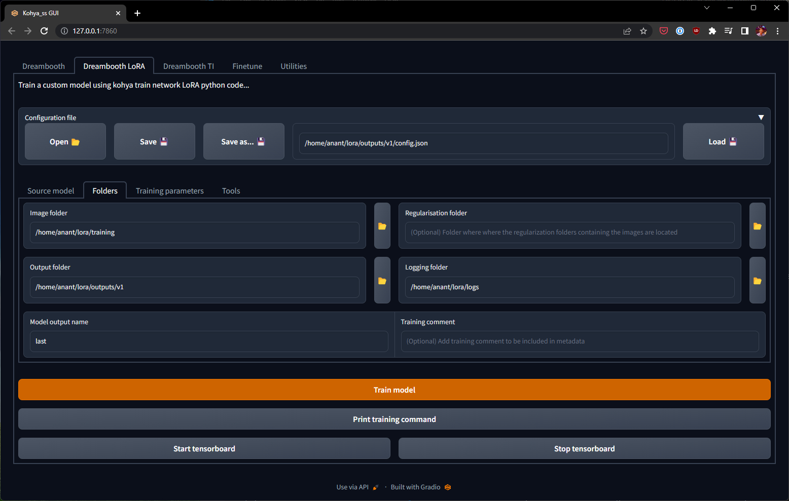 Folder configuration
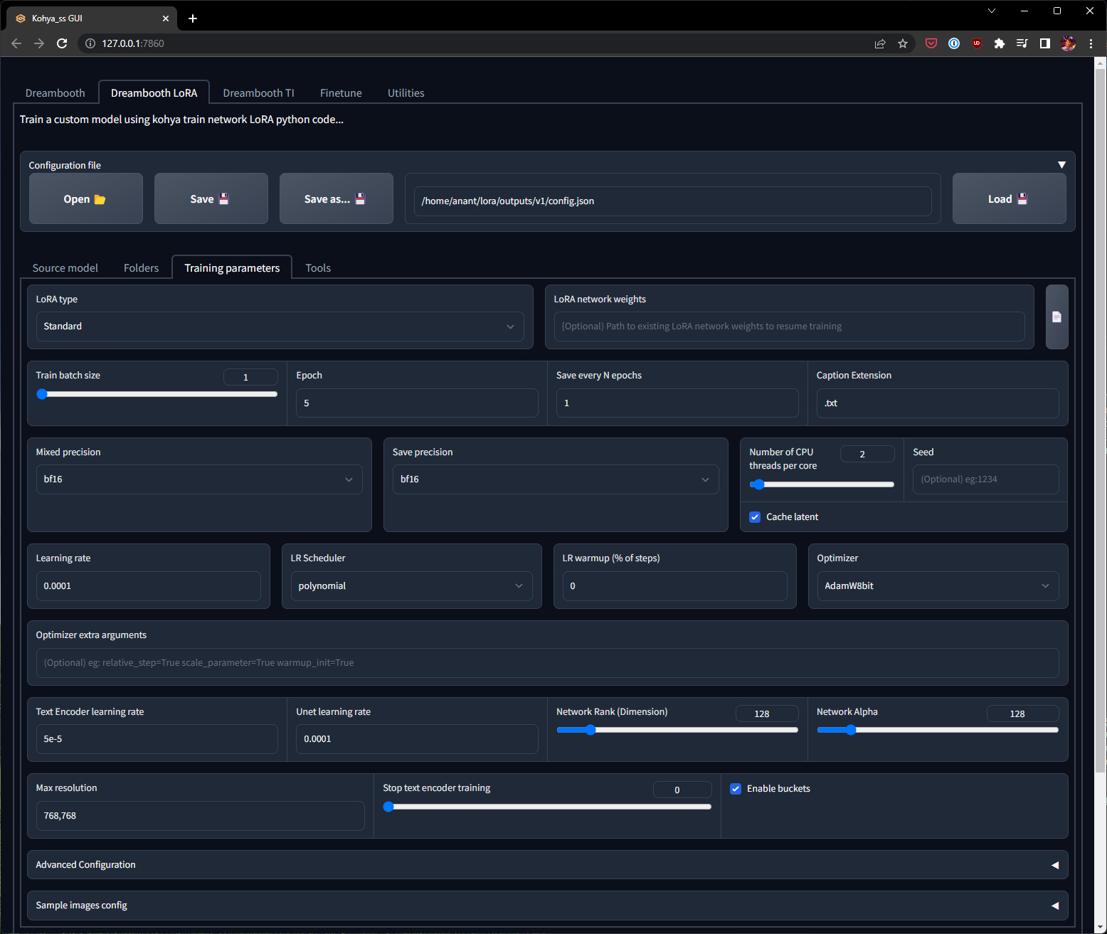 Hyperparameter configuration
Double check all the values again. Couple of more settings to keep in mind:
- Don’t forget to set the “Caption extension” value to
.txt! - For max resolution, if most of your images are larger than 768x768, then you can set
768,768as the value. If not, leave it at the default512,512.
Click the “Train model” button, and wait for the training to complete. You can follow progress on the terminal where you started kohya_gui.py. For 1875 steps on my RTX 4090, this took less than 10 minutes.
Testing
Now comes the fun part! Let’s test our model to see how we did.
For testing, I used Protogen x5.3, which is a fine-tuned derivation of Stable Diffusion v1.5. You can certainly use the plain v1.5 model, but models like Protogen give you a lot more creative tools and prompting options.
To use a model like Protogen, just download the safetensors file from HuggingFace and place it in the models/Stable-diffusion/ directory in your Automatic1111 installation. At this point, also copy (or symlink) the output of your LoRA fine-tuning run into models/Lora/. The directory structure inside stable-diffusion-webui should now look something like this:
|- models
|  |- Lora
|  |  |- last-000001.safetensors
|  |  |- last-000002.safetensors
|  |  |- last-000003.safetensors
|  |  |- last-000004.safetensors
|  |  |- last.safetensors
|  |- Stable-diffusion
|  |  |- ProtoGen_X5.3.safetensors
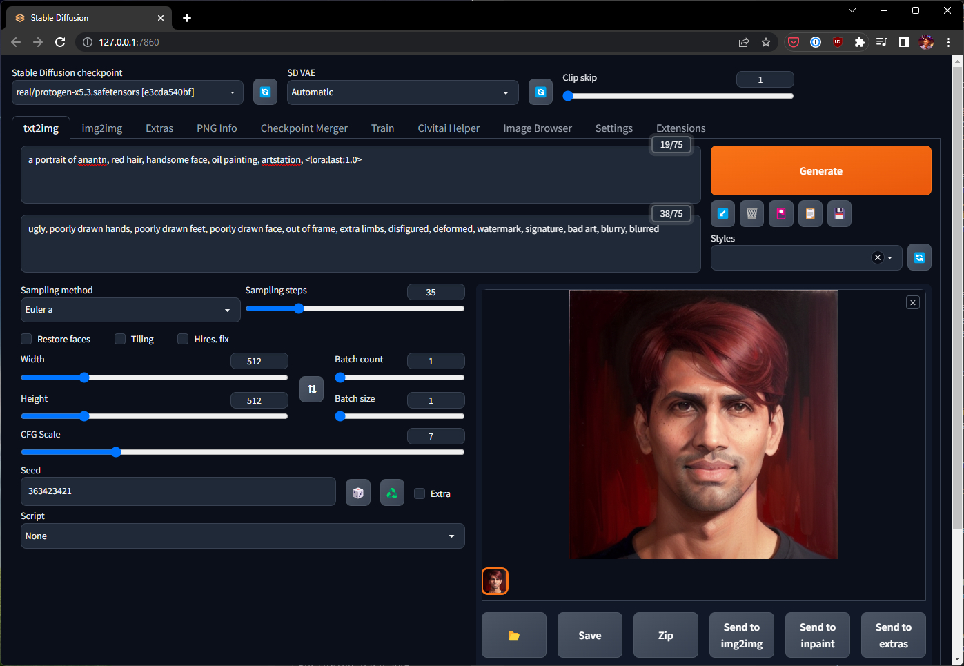
Fire up launch.py (see my installation post for the best command-line arguments) and think of your test prompt. I chose something like:
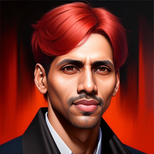
a portrait of anantn, red hair, handsome face, oil painting, artstation, <lora:last:1.0>
Negative prompt: ugly, poorly drawn hands, poorly drawn feet, poorly drawn face, out of frame, extra limbs, disfigured, deformed, watermark, signature, bad art, blurry, blurred
Steps: 35, Sampler: Euler a, CFG scale: 7, Seed: 363423421, Size: 512x512
You’ll obviously want to swap out the token anantn for whatever value you used during training. Click generate! If all went well you should see an oil painting of someone with your likeness with red hair 😊
Testing tips
Here are a few guidelines to keep in mind as you test your newly baked LoRA!
X/Y/Z Plots
This is a very handy feature in Automatic1111 that lets you generate batches of images varying some aspect of your prompt. In the prompt we used above, the token <lora:last:1.0> referred to only the last epoch at full strength. Varying this value through an X/Y plot can help you understand how training progressed and if a different epoch at a different strength produced more desirable results.
To generate something like that, just select “X/Y/Z plot” from the drop-down in “Script”. For “X type”, and “Y type” select “Prompt S/R”, which stands for Prompt Search/Replace.
- Set “X values” to
last, last-000001, last-000002, last-000003, last-000004 - Set “Y values” to
1.0, 0.9, 0.8, 0.7, 0.6, 0.5
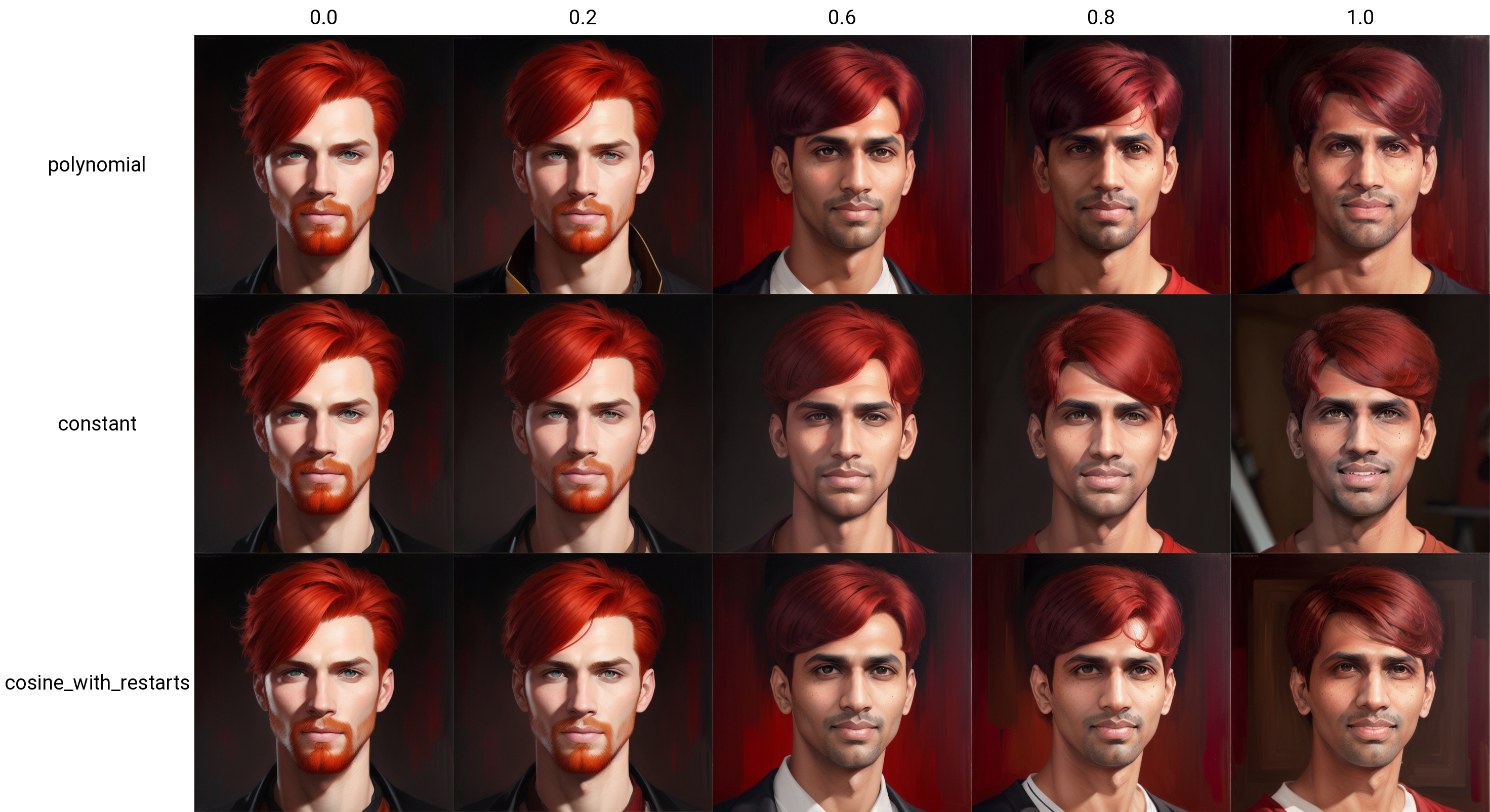
This will cycle through all epochs you trained as well as give you a sense of how applying the LoRA at different strengths affects the output. I used X/Y/Z plots extensively to compare outputs not just between epochs, but also between different hyperparameter configurations. For example, here is an X/Y plot that compares the polynomial, cosine_with_restarts, and constant scheduler type at various strengths:
Underfit or overfit?
What you look for in a good LoRA can depend a lot on your particular training set and your own artistic sensibility. In my specific case, I was really looking for two main things:
- Likeness: the output should look like me! I comb my hair somewhat unconventionally, from right to left, the model picking up on that was a good sign that it picked up my likeness. Note how in the grid above, the combing direction changes at strength
1.0forpolynomialand0.8forconstant. - Adaptability: an easy test was to see if the model could turn my (naturally black) hair into a bright red color. Hair turning blackish even though my prompt says red hair is a sign of overfitting. There can be other signs too, such as at strength
1.0inconstant, you can see elements in the background that are from my training set but not my prompt.
It might be helpful for you to identify your own criteria based on details of your likeness and face, both on the low end (turning a stock image into your likeness) and on the high end (outputs looking too similar to training data, losing prompting flexibility).
 AdaFactor produced underfit: likeness not strong enough, beard still present
 Constant with high LR produced overfit: background is smudged
Generalizability
Once you have found a particular epoch and strength that you like on a simple prompt like the one above — you can move onto to testing the flexibility and generalizability of your LoRA.
A good LoRA will give you good results in a variety of conditions; I encourage you to experiment with things like varying hair colors, adding accessories, changing outfits, and trying out both artistic and realistic environments and backgrounds. Here are a few that I tried:
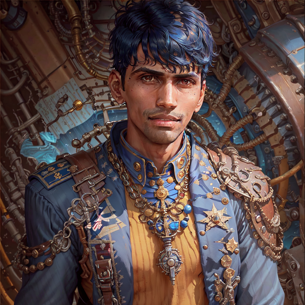 In military uniform, steampunk style
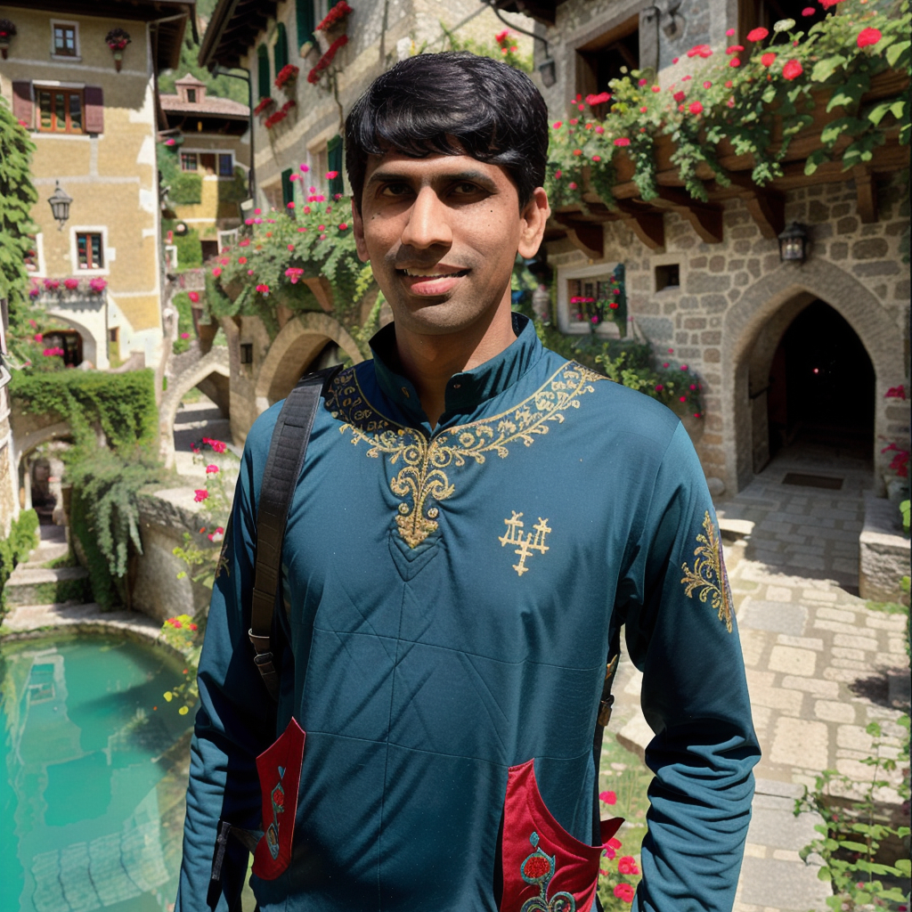 Realistic, jester clothes, swiss town
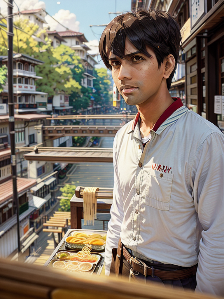 Working in a ramen shop, as a boy
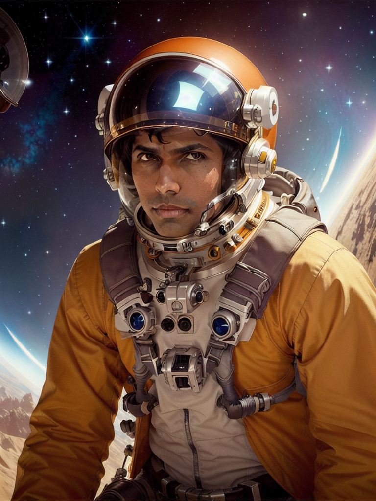 In an astronaut suit
I’m pretty pleased with the results - this feels like a solid, baked, generalizable LoRA 👍 While I was a happy “Magic Avatars” customer, these results far surpass what I got back from most commercial services offering AI-generated avatars! And I can generate a near-infinite number of these, limited only by my imagination and prompt-writing ability.
Keep in mind the work shown in this post took me several tries over several days to achieve successful results. If you didn’t get great results on your first attempt, go back to the section on hyperparameter selection and see if tweaking these values helps. I’d also encourage keeping a training diary to keep track of your experiments and results.
Objects & Styles
Now that you have a repeatable process for creating new LoRAs, you can try them for different characters, objects, and styles. Applying the same process to a training set consisting of photos of my dog, I got impressive results:
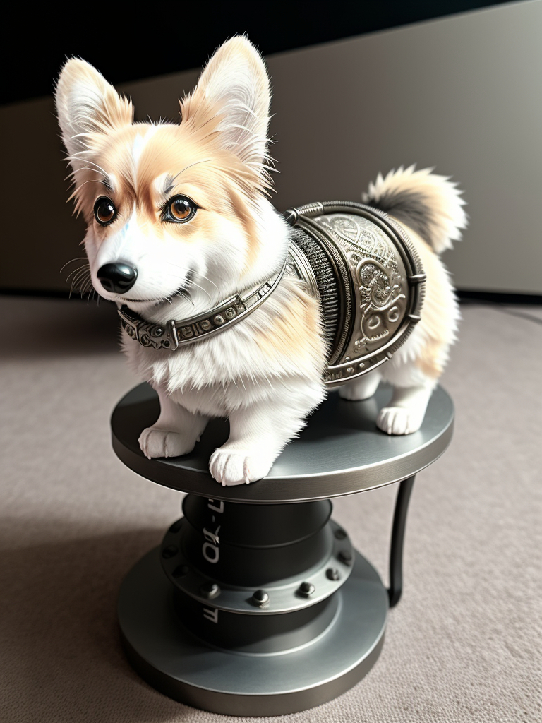 Wearing metallic armor
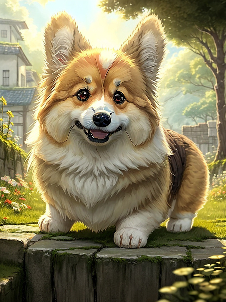 Ghibli style
My friend Vikrum had an awesome idea to create art resembling the style found on Indian trucks. This art style is quite unique, but very niche and hence not present in any mainstream image generation model. The ubiquitous phrase “Horn OK Please” is painted on the back of nearly every truck in India, surrounded by art in a distinctive style.
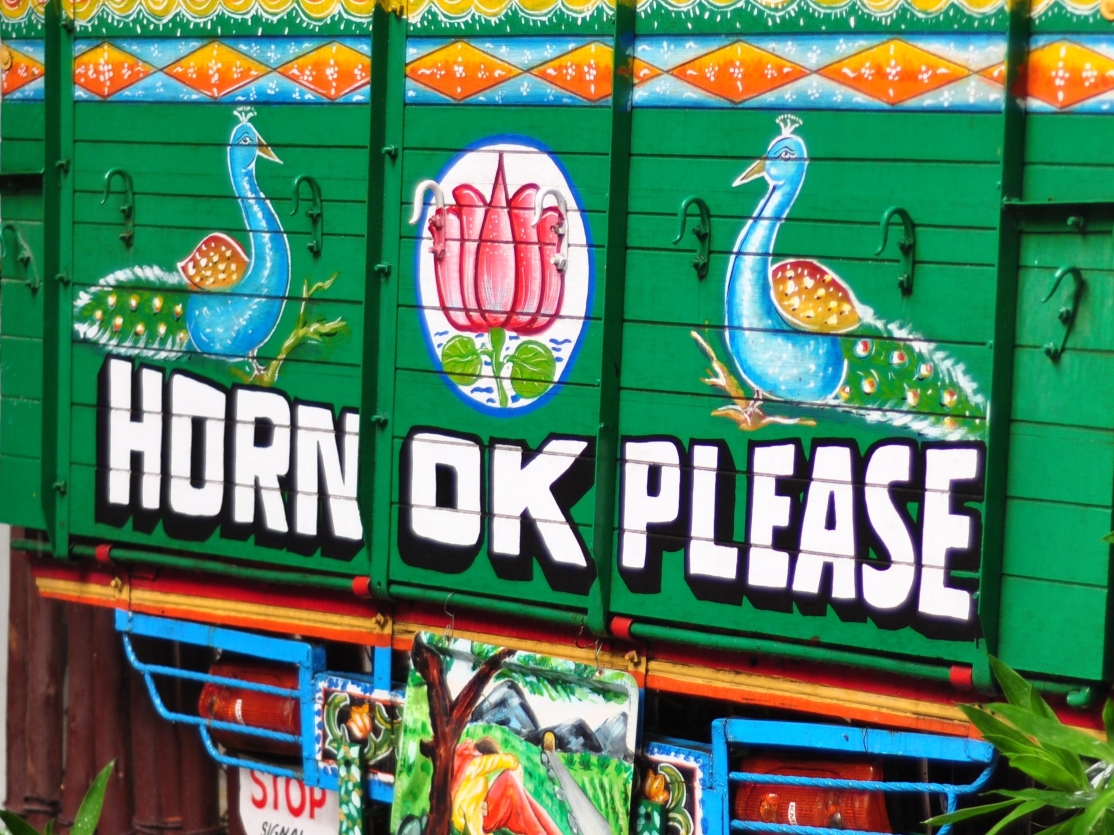 Typical art style found on the back of Indian trucks
We had trouble reproducing this style in Midjourney, but that makes it a perfect use-case for LoRAs with Stable Diffusion. Once again, following the process above, we produced a LoRA that can represent any concepts in the style of Indian truck art:
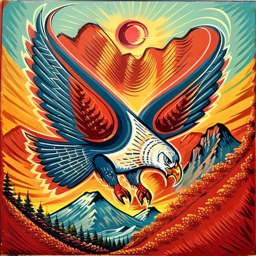 American bald eagle in Indian truck style
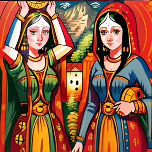 Mona Lisa in Indian truck style
This LoRA was trained with only 30 training images; I suspect we can do substantially better with more training data. Anecdotally, styles transfer best at 100+ training images. Here is a reddit post on creating a style LoRA based on the Artist Photoshop effect, which could be another good resource.
LyCORIS (LoCon / LoHa)
There have been some extensions to the core LoRA algorithm, called “LoCon” and “LoHA”, which you might see in the dropdown options in the kohya_ss GUI. These are built on the learning algorithms in this repository.
I gave these a try but was unable to reproduce results that got anywhere close to the quality of the original LoRA — even with the suggested parameters of <32 dimensions and low alpha (1 or lower). It’s worth keeping an eye on these methods as they evolve, but for now I suggest sticking with conventional LoRA.
Summary
LoRA is a powerful and versatile fine-tuning method to create custom characters, objects, or styles. While the training data and captioning process is rather cumbersome today, I imagine large parts of this process will be automated to a great degree in the coming months. It wouldn’t surprise me to see many LoRA-based commercial applications pop up in the near future.
Let me know how this method worked for you, or if you have any questions or comments on the process!